Different types of real numbers(denoted by the symbol ) were invented to meet specific needs. Rational numbers are constructed by taking ratios of integers, thus any rational number is expressed as
Real numbers such as cannot be expressed this way and are therefore called irrational numbers. Rational numbers’ corresponding decimal representations are repeating. For example,
To convert a repeating decimal to a ratio of two integers, we can eliminate the repeating part by multiplying it to appropriate powers of 10 then subtract. For ,
Thus .
For any real number , we have , therefore the number is called the additive identity and the number is called the multiplicative identity. is the inverse of any real number that satisfies , similar to how division undoes multiplication:
Recall that we refer to as the quotient of and or as the fraction over ; is the numerator and is the denominator or divisor.
We rewrite fractions so that they have the Least (smallest possible) Common Denominator (LCD) when adding fractions with different denominators. For example, evaluate: .
First, factor each denominator into prime factors:
Then, find the LCD by forming the product of the highest power occurred of each of the prime factors, in this case, . So
To express positive number in scientific notation:
The exponentindicates how many places the decimal points should be moved. For instance,
The symbol means the positive (principal)square root of, thus
The same applies to the principal th root, and if is even, and . For instance, is not defined.
For any rational exponent (), we define
It is often useful to rationalize the denominator, making the fractional expression to be in standard form, by multiplying both the numerator and the denominator by an appropriate expression. In general, with and the denominator being of the form , multiple by rationalizes the denominator:
With , creates a negative exponent which may lead to a reciprocal so we often use another method for clarity. Take as the quotient of and as the remainder, recall that
Then
So naturally,
In this case, the expression to multiply by is .
When comparing roots, multiply the rational exponents by their LCD. For instance,
Expressions
An algebraic expression combines real numbers and variables. A monomial is an expression of the form , where the coefficient is a real number and is a nonnegative integer, while a polynomial is a sum of monomials called terms of the form
The degree of the polynomial is the highest power of the variable appears. The number is the leading coefficient and the term is the leading term.
Use the Distributive Property to expand algebraic expressions, and reverse the process by factoring them. To factor a trinomial of the form , note that
so find the numbers that satisfy , and .
A trinomial is a perfect square if it is of the form , and can be recognized by checking if the middle term is twice the product of the square roots of the outer terms. For instance, notice that . The technique of completing the square is used to make a perfect square. To make a perfect square, add :
Factor the coefficient of first if it isn’t .
These special factoring formulas need to be memorized:
When factoring expressions with fractional exponents, try to factor out the smallest exponent, for instance
Rational expressions are fractional expressions, which can be simplified by cancelling common factors. To simplify a compound fraction in which the numerator or the denominator is a fractional expression, multiply by the LCD of all the fractions. For instance,
The form can be rationalized by multiplying by the conjugate radical:
Equations
An equation is a statement of equality of two mathematical expressions satisfied by its solutions. Equivalent equations share the same solutions, and solving an equation is to find the equivalent equation in which the variable stands alone on one side.
Linear equations or first-degree equations has each term being either a constant or a nonzero multiple of variable. With one variable, it is of the form . Quadratic equations are second-degree equations of the form . Complete the square to find a formula for its solution:
The quantity under the square root is the discriminant.
Using LCD to factor equations can be efficient. For instance, to solve , multiply by LCD and it’s immediately factored to a general quadratic equation.
Operations such as multiplying by an expression with variables or squaring (a radical) may turn a false equation into a true one and therefore introduce extraneous solutions, so alwayscheck the answers to make sure each satisfies the original equation.
Complex Numbers
The complex number system is an expanded number system. We define
And for any negative number , similar to how positive real number has two square roots , its square roots are , and the principal square root is .
A complex number is an expression of the form . The real part of the complex number is and the imaginary part is which are both real numbers. A pure imaginary number has a real part of . Notice that
For , we define its complex conjugate to be , so
which is always a nonnegative. This property is used to divide complex numbers:
To prove some other properties of complex conjugates:
Also notice that if complex number is real, meaning and , we can write .
In the complex number system, a quadratic equation always have solutions, even when the discriminant , in which case the solutions are complex conjugates of each other:
We define the length (or magnitude) of a complex number as
Notice
So the square of the length of a complex number is the product of the complex number and its complex conjugate:
By the way,
Inequalities
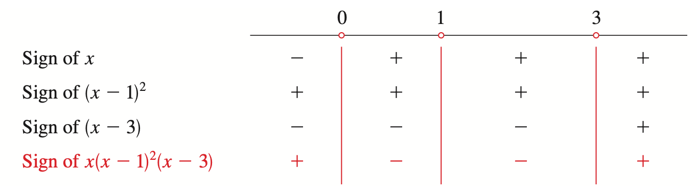
Unlike an equation, an inequality generally has infinitely many solutions. To solve nonlinear inequalities involving squares and other powers of the variable, factor and determine the values for which each factor is zero, which divide the real line into intervals. Test and make a table or diagram of the signs of each factor on each of the intervals, and finally determine the sign of the product of the factors. Check the endpoints.
For instance, to solve , first divide the real line into intervals based on the values for which each factor is zero:
Make the following diagram:
The solution set is clearly the union of two intervals: . Same applies to inequalities involving quotients, for instance, evaluate :
The factors are and , so we divide the real line into the intervals
and so on.
Graphs
Like points on a line identified with real numbers form the coordinate line, points in a plane form the coordinate plane, in which any point can be located by a unique ordered pair of numbers . is the x-coordinate and is the y-coordinate. The formula to find the distance between two points and is
The graph of an equation in and is the set of all points that satisfy the equation, we can sketch a graph by plotting points. Conversely, we can find an equation of a graph that represents a given curve in the -plane. The rules of algebra can be used to analyze the curve. For instance, a circle with radius and center is the set of all points which is on the circle if and only if
We can complete the square when given the equation of a circle in expanded form to get the standard form.
Lines
The slope of a nonvertical line that passes through and is defined as
and for any point that lies on this line, by definition,
This is the point-slope form of the equation of a line.
If a nonvertical line has slope and -intercept , it intersects the -axis at , the point-slope form simplifies to
which is called the slope-intercept form of the equation of a line.
A linear equation in and , which is the general equation of a line, is of the form
A nonvertical line has the equation , in which , and , or conversely
If the - and -intercepts of a line are nonzero numbers and , meaning the line intersects the axes at and , the slope of the line is , so the equation can be written in the form
This is called the two-intercept form of the equation of a line.
Consider two lines with equations and which vertical line intersects at and , notice that if and only if
Two lines are perpendicular if and only if their slopes are negative reciprocals.
Modeling Variation
A mathematical model is often an equation or formula that describes the relationship of one physical quantity to another.
A direct variation occurs when one quantity is a constant multiple of the other:
We say varies directly as, or is (directly) proportional to. The constant is called the constant of proportionality.
A inverse variation is when the quantities are related by the equation
We say varies inversely as, or is inversely proportional to.
Many laws of nature are inverse square laws. A quantity(force or energy) originating from a point source spreads its influence equally in all directions, and at a distance , it is spread out over the surface of a sphere of radius , which has area, so the intensity is source strength divided by that area
much like the Law of Gravity
Functions
A function is a rule that assigns exactly one element , called the value of at or the image of under , read ” of/at ”, to each element in the domain of the function. Unless explicitly defined, the domain of a function is the domain of the algebraic expression–the set of all real numbers for which the expression is defined.
When we write , the symbol is the independent variable and is the dependent variable which represents a number in the range of .
Any equation in the variables and defines a relationship between them, but not every equation defines as a function of , for example,
which gives two values of for a given value of .
Many properties of a function can be obtained from the graph. The function is said to be increasing on an interval if and is said to be decreasing if whenever in . The function value is a local maximum value of if and is a local minimum value of if , when is near . is a local maximum point and is a local minimum point and these points are called the local extrema of the function.
Certain transformations of a function affect its graph:
An even function satisfies which graph is symmetric with respect to the -axis, and an odd function satisfies which graph is symmetric with respect to the origin.
Functions may be combined algebraically to form new functions with the domain being the intersection of the domains of the combined functions.
its inverse function is defined by which reverses the effect of. To find the inverse of a function , solve the equation for in terms of and interchange and , resulting . The graph of is obtained by reflecting the graph of about the line .
and are inverses of each other. satisfies the following cancellation equations:
This can be used to verify if two functions are inverses of each other. For example, and are inverses because
Polynomial Functions
The graph of any quadratic function is a parabola which can be obtained from the graph of by transformations, we can also complete the square to express the a quadratic function in the vertex form
with the vertex of the parabola being . is the minimum value if and the maximum value if .
Generally, we refer to polynomial functions as simply polynomials, the simplest of which are the monomials , whose graphs has the same general shape as the graph of when is even and the same general shape as the graph of when is odd. The greater the degree of a polynomial, the more complicated its graph can be, but its end behavior is always determined by the leading term which contains the highest power of .
is called a zero of polynomial if which would also be an -intercept at . The intermediate value theorem suggests there exists at least one zero in if and have opposite signs. As a consequence, the values between two successive zeros are either all positive or all negative. Use zeros to determine the intervals, then test points in the intervals to graph the polynomial.
Generally, if is a zero and the corresponding factor occurs times in the factorization, we say is a zero of multiplicity. If is even, meaning the factor is raised to an even power, it doesn’t change sign as we test points on either side of , so the graph does not cross the -axis at . The graph does cross the -axis at if multiplicity is odd. It can be shown using calculus that the graph has the same general shape as near .
(Calculus) A polynomial of degree can have at most distinct real roots, so its derivative which has degree can have at most zeros, each zero is a possible place for a local extrema of the polynomial. Therefore, a polynomial of degree can have at most local extrema.
When dividing by , the quotient is and the remainder is , we write:
Similarly, if and are polynomials with , there exist unique polynomials and such that
The remainder is either or of degree less than the degree of , and as a consequence, if the divisor is of the form , the remainder must be a constant:
Notice . This is the remainder theorem: if the polynomial is divided by , the remainder is the value . And, if is a zero of , meaning , then has to be a factor of . When the divisor is of the form , use synthetic division(see textbook page 277) to divide the polynomial.
Specifically, if polynomial has only integer coefficients, and is a rational zero of , in lowest terms, we have
This says is a factor of constant and is a factor of the leading coefficient since is in lowest terms and therefore and have no factor in common. This is the rational zeros theorem, from which we can see if the leading coefficient is or , then all rational zeros of the polynomial must be factors of the constant term. For example, for , the possible rational zeros are of the form , so , , , , and . It is possible to find all rational zeros by testing each of these possibilities, but it would be easier to use synthetic division to check these possible zeros because upon finding an actual zero(that is, when we get a remainder of ), we get the factored form of the polynomial automatically.
Descartes’s rule of signs is helpful in eliminating candidates from lengthy lists of possible rational roots in some cases. A variation in sign occurs whenever adjacent coefficients have opposite signs. The rule says:
The number of positive real zeros in either is equal to the number of variations in sign in or is less than that by an even whole number.
The number of negative real zeros in either is equal to the number of variations in sign in or is less than that by an even whole number.
For example, to evaluate , since has variation in sign and has , has positive real zero and or negative real zero(s).
The upper and lower bound for the zeros of a polynomial can be found by dividing it by
(with ), and if the quotient and remainder has no negative entry, is an upper bound for the real zeros of
(with ), and if the quotient and remainder has alternately nonpositive and nonnegative, is a lower bound for the real zeros of , can be considered to be positive or negative as required
For example, to show that all the real zeros of lie between and , divide it by and using synthetic division and confirm the entries. Additionally, always check the entries when using synthetic division to factor polynomials of high degrees to eliminate impossible candidates.
Recall that quadratic equations always have solutions in the complex number system. Generally, the Fundamental Theorem of Algebra states that every polynomial has at least one complex zero because there must exist some complex number such that the magnitude (note that any real number is also a complex number). As a consequence, the polynomial can be factored completely by repeating the process:
Therefore we conclude that in the complex number system, any polynomial with degree of has exactly zeros(counting multiplicities), meaning it can be factored into exactly linear factors. This is the complete factorization theorem.
If the polynomial has real coefficients, and suppose that complex number is a zero, so , recall the properties of complex conjugates, we have
This shows the complex conjugate would also be a zero of . This is the conjugate zeros theorem: complex roots occur in conjugate pairs. This would not apply if has complex coefficients. Observe that if is a complex number, then
which is a quadratic with real coefficients. Multiply the factors corresponding to each such pair of any such polynomial and we get a quadratic factor. A quadratic polynomial with no real zeros is called irreducible over the real numbers. Therefore, even if we don’t use complex numbers, every polynomial can still be factored into a product of linear and irreducible quadratic factors. This is the linear and quadratic factors theorem.
Rational Functions
Rational functions are of the form
where and are polynomials. The convention is that and have no factor in common, and if they do, we may cancel the common factors for those values of for which that factor is not zero, at which point the function is not defined:
Linear fractional transformations are rational functions of the form
Notice that linear expressions can always be rewritten in terms of another linear expression. In general,
where and . Notice that the two lines, and must not be proportional (linearly dependent), so , or, for general validity, we prefer to write it as . Otherwise would be a constant.
Thus can be rewritten as
This shows a linear fractional transformation can always be graphed by transforming the graph of which behavior can be described using arrow notation:
Notice the symbols and meaning ” approaches from the left or the right”. is a vertical asymptote of because approaches as approaches , and is a horizontal asymptote because approaches as approaches . Shifting the graph of a rational function vertically shifts the horizontal asymptotes; shifting the graph horizontally shifts the vertical asymptotes: has vertical asymptote and horizontal asymptote .
We analyze other types of rational functions in similar fashion. For any rational function
The vertical asymptotes are determined by the zeros of the denominator, and the horizontal asymptotes are determined by the leading terms, because after dividing both the numerator and denominator by an appropriate power of , most terms approach as .
A rational function of the form with the degree of being one more than the degree of can be expressed in the form
Notice that because the degree of the remainder is less than the degree of the divisor , as . In this situation we say is a slant asymptote. There are also end behaviors other than horizontal and slant asymptotes depending on what we get after division. For example, using synthetic division,
as , so the end behavior is like that of the parabola .
Rational functions are not necessarily continuous, unlike polynomials. As consequences, to determine the intervals on which a rational function does not change sign, we need to look at its cut points, which are not only its zeros, but also the vertical asymptotes, that is, the values of at which either or .
Exponential Functions
The exponential function with base is defined for all real numbers , including when is irrational which can be approximated by rational numbers intuitively, by
is assumed because it would otherwise make a constant function.
Compound interest is calculated by the formula
where is the principal, is the annual interest rate and is the number of times interest is compounded annually.
The number is a special base defined as the value that approaches as becomes large. It can be shown that which is an irrational number. The exponential function with the base is the natural exponential function.
If we let , we have
increases as the number of compounding periods increases, and the quantity approaches the number . Thus continuously compounded interest is calculated by the formula
The inverse function of every exponential function is called the logarithmic function with base , denoted by , is defined by
Thus is the exponent to which the base must be raised to give .
It is important to see the logarithmic form as an exponent.
The logarithm with base is called the common logarithm and is denoted by emitting the base: . The logarithm with base is called the natural logarithm and is denoted by : .
When solving exponential equations, isolate the exponential expression on one side, then take logarithm of each side. For example,